Wolfram Mathematica How to Make X Become X Again
Function I: Plotting
This tutorial contains many Mathematica scripts. You, as the user, are free to use all codes for your needs, and have the right to distribute this tutorial and refer to this tutorial as long as this tutorial is accredited accordingly. I would like to extend my gratitude to all of the students that aided me in developing this tutorial. The coding, testing, and debugging required a concerted effort, and the following students deserve recognition for their input: Emmet and Jesse Gilt-Marx (Fall 2011), Pawel Golyski (Fall 2012). Any comments and/or contributions for this tutorial are welcome; you tin ship your remarks to <Vladimir_Dobrushkin@brownish.edu>
Return to computing page for the first class APMA0330
Return to computing page for the second class APMA0340
Return to Mathematica tutorial page for the first course
Return to Mathematica tutorial page for the second course
Render to the main page for the form APMA0330
Return to the main folio for the form APMA0340
1.one. Plotting functions
Ane of the best characteristics of Mathematica is its plotting ability. Information technology is very piece of cake to plot a multifariousness of functions using Mathematica. For a plot, information technology is necessary to define the contained variable that you are graphing with respect to. Mathematica automatically adjusts the range over which you are graphing the function.
Plot[2*Sin[3*x]-2*Cos[x], {x,0,2Pi}]
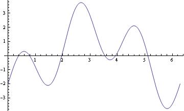
In the in a higher place code, we use a natural domain for the independent variable to be \( [0,two\pi ] .\) In full general, the domain of the contained variable is usually called based on a particular involvement; one may try different options before obtaining a desired figure.
Plot[{Cos@x, ArcCos@ten}, {x, -Pi, Pi}, PlotStyle -> Thick]
In this command sequence, the independent variable is ten and the range is 0 to \( 2\pi .\) For Plot, after entering the office that y'all wish to graph, you separate the equation and add {independent variable, lower bound, upper bound}.
This is a simple Plot control. In this example, we are just plotting a function using Mathematica default capabilities, but it is possible to specify the range with PlotRange command. The above graph can also be obtained with the following script:
Plot[2*Sin[3*x]-2*Cos[ten], {x,0,2Pi}, PlotRange -> Automatic]
To identify a text inside a effigy, Mathematica has a special command Text[expr, coordinates, start] that specifies an offset for the block of text relative to the coordinate given. Providing an offset { dx, dy } specifies that the bespeak ( x, y ) should prevarication at relative coordinates { dx, dy } inside the bounding rectangle that encloses the text. Nosotros demonstrate it with the following codes:
Plot[Sin[x] - Cos[iii*x]/3, {x, 0, three},
Epilog -> {Text[Fashion["hullo", 25], Scaled[{0.5, 0.5}], #], Crimson, Point@{.v, .five}},
PlotLabel -> ToString@#] & /@ {{-2.5, 0}, {2.5, 0}, {0, -2}, {0, 2}, {two, 2}, {-3, -2}}
However, when we modify dimensions of the graph, the text is displayed differently.
Plot[Sin[x] - Cos[3*x]/three, {x, 0, 3},
Epilog -> {Text[Way["hullo", 25], Scaled[{0.v, 0.5}], #], Blood-red, Point@{.five, .5}},
PlotLabel -> ToString@#] & /@ {{-2.5, 0}, {2.v, 0}, {0, -2}, {0, 2}, {two, ii}, {-3, -2}}
The following tabular array of graphs can exist displayed using GraphicsGrid command. GraphicsGrid by default puts a narrow border around each of the plots in the array it gives. You can alter the size of this border by setting the option Spacings -> { h, v} . The parameters h and v give the horizontal and vertical spacings to exist used. The Spacings option uses the width and height of characters in the default font to calibration the h and v parameters by default, just it is generally more useful in graphics to utilize Scaled coordinates. Scaled scales widths and heights then that a value of i represents the width and height of ane chemical element of the filigree.
How to add text to a graph, see
http://reference.wolfram.com/linguistic communication/howto/AddTextToAGraphic.html.en
To add test outside the flick, see
http://reference.wolfram.com/language/howto/AddTextOutsideThePlotArea.html.en
The general reference is
http://reference.wolfram.com/linguistic communication/howto/AddTextToAGraphic.html
On most reckoner systems, Mathematica can produce not simply graphics only also sound. Mathematica treats graphics and sound in a closely analogous way, using command Play. For case, the previous function can be used to play, on a suitable figurer arrangement, a pure tone with a frequency of 440/2π hertz for one 2d.
Play[2*Sin[3*x*440] - 2*Cos[10*440], {x, 0, 1}]
For multiple plots, apply either command Show or you lot can use {} with commas. Show can be used to change the options of an existing graphic or to combine multiple graphics.
Plot[{ii Sin[3 x] - 2 Cos[x], Sin[10] - 1/three Cos[3 x]}, {x, 0, iii}, PlotStyle -> Thick]

Show command can be used to accommodate the Background choice of an existing graphic
g1 = Plot[Sin[x] - i/3 Cos[3 x], {ten, -ane, 3}, PlotStyle -> Thick]
Show[{g1, Graphics[Circle[]]}, Background -> Yellow, AspectRatio -> Automatic]

A graphic of a part can be fabricated discrete:
Graphics[{Blue,
Indicate[Table[{x, Sin[x] - 1/3 Cos[3 ten]}, {ten, 0, 6, .2}]]}, Axes -> Truthful]

Nosotros can shift the origin to another indicate, as the post-obit example shows.
g1[x_] = Sin[x] - 1/3 Cos[3 x]
g1[0]
Out[3]= -one/3
bp = Plot[g1[10], {x, 0, 6}]
Bear witness[bp, AxesOrigin -> {0, -one/3}, AxesLabel -> {"x", "y"}]

When you need to restrict the vertical range, use PlotRange control equally the following instance shows.
Plot[(10 - one)*(10 - ii)*(x - iii)*Exp[x], {x, -v, 3.5}, PlotStyle -> {Black, Thick},
AxesLabel -> {ten, (x - i)*(x - two)*(x - 3)*Exp[x]}]
Plot[(x - 1)*(x - 2)*(x - three)*Exp[10], {x, -v, 3.five}, PlotRange -> {-5, 8},
PlotStyle -> {Black, Thick}, AxesLabel -> {x, (x - 1)*(x - ii)*(x - three)*Exp[x]}]
Plot sine function downward:
data1 = Table[{x, Sin[10]}, {x, -v, 5, 0.1}];
ListLinePlot[data1, PlotRange -> All];
ticks = Table[{-10, 10}, {x, -v, five, .2}];
ListLinePlot[{#, -#2} & @@@ data1, PlotRange -> {All, i}, Ticks -> {All, ticks}, Axes -> True, PlotStyle -> Thick]

data1 = Table[{x, Sin[x]}, {ten, -5, 5, 0.1}];
ListLinePlot[data1, PlotRange -> All];
ticks = Table[{-x, x}, {x, -5, v, .2}];
ListLinePlot[{#, -#2} & @@@ data1, PlotRange -> {-1.3, one.3},
Ticks -> {All, ticks}, Frame -> False, PlotRange -> All,
Epilog -> {Text["ten", {5.5, 0}], Text["y", {0, -1.4}]},
PlotRangeClipping -> False, ImagePadding -> {{20, twenty}, {20, 20}}]

Now plot with arrows, only without units:
axes[x_, y_, f_, a_] :=
Graphics[Bring together[{Arrowheads[a]},
Arrow[{{0, 0}, #}] & /@ {{x, 0}, {0, y}}, {Text[
Mode["x", FontSize -> Scaled[f]], {0.95*x, 0.1*y}],
Text[Style["y", FontSize -> Scaled[f]], {0.1 x, 1*y}]}]]
data1 = Table[{x, Sin[x]}, {x, 0, 5, 0.1}];
ListLinePlot[data1, PlotRange -> All];
ticks = Table[{-x, x}, {x, -5, 5, .2}];
Show[ListLinePlot[{#, -#ii} & @@@ data1, PlotRange -> {-1.three, 0},
Ticks -> {None, None}, Frame -> False, PlotRange -> All,
PlotRangeClipping -> Fake, ImagePadding -> {{20, twenty}, {20, 20}}],
axes[5.iii, -1.33, .06, .05], Axes -> Simulated]

Example. Tractrix (from the Latin verb "trahere" -- pull, drag; plural: tractrices) is the bend along which an object moves, under the influence of friction, when pulled on a horizontal plane by a line segment attached to a tractor (pulling) point that moves at a correct angle to the initial line betwixt the object and the puller at an infinitesimal speed. Past associating the object with a domestic dog, the string with a leash, and the pull along a horizontal line with the domestic dog's principal, the curve has the descriptive proper name hundkurve (dog curve) in German language. It is therefore a curve of pursuit. It was offset introduced by Claude Perrault (1613 -- 1688) in 1670. Trained as a physician, Claude was invited in 1666 to become a founding member of the French Academie des Sciences, where he earned a reputation as an anatomist. The first known solution was given by Christian Huygens (1692), who as well named the curve the tractrix. Its parametric equation is
\[ 10 = a\, \sin (t), \qquad y = a\left( \cos (t) + \ln \left(\tan (t/ii)\right) \right) . \]
To plot tractrix curve, we use the following lawmaking:
tractrix[a_][t_] := a*{Sin[t], Cos[t] + Log[Tan[t/2]]};
Dispense[
ParametricPlot[tractrix[a][t] // Evaluate, {t, 0, .99*\[Pi]},
PlotRange -> {0, vii}], {a, 1, 6}]
Export["tractrix1.gif",%]

Manipulate[
Plot[y'[x] = -Sqrt[a^two - x^ii]/10, {x, 0, twenty},
PlotRange -> {-10, 10}], {a, 0, 20}]

sol = DSolve[{y'[x] == -Sqrt[a^two - ten^2]/10, y[a] == 0}, y, x]
Out[2]= {{y -> Function[{x}, -Sqrt[a^two - x^2] + a Log[a] - a Log[a^two] -
a Log[x] + a Log[a^2 + a Sqrt[a^two - ten^ii]]]}}
Dispense[
Plot[-Sqrt[a^2 - x^ii] + a Log[a] - a Log[a^2] - a Log[x] + a Log[a^2 + a Sqrt[a^2 - 10^2]], {ten, 0, xx}, PlotRange -> All], {a, 1, 20}]

Return to the chief page (APMA0330)
Return to the Office two (First Club ODEs)
Return to the Role 3 (Numerical Methods)
Return to the Office four (Second and College Club ODEs)
Return to the Office 5 (Series and Recurrences)
Render to the Part vi (Laplace Transform)
Render to the Office 7 (Boundary Value Problems)
Source: https://www.cfm.brown.edu/people/dobrush/am33/Mathematica/part1.html
0 Response to "Wolfram Mathematica How to Make X Become X Again"
Post a Comment